133.1x: Confined flow with precipitation#
Transient solution (133.16)#
This notebook shows the Bruggeman solution for:
One dimensional finite flow. Given head or drawdown at x=b and zero flux at x=0.
Steady state (133.17) shown as well.
import matplotlib.pyplot as plt
import numpy as np
import timflow.transient as tft
from numpy import linspace

from bruggeman.flow1d import bruggeman_133_16, bruggeman_133_17
bruggeman_133_16
\[\begin{split}
\begin{aligned}
\beta &= \sqrt{\frac{S}{D k}} \\
\varphi{\left(x,t,b,S,k,D,p,N \right)} &= - \frac{16 b^{2} p \sum_{n=0}^{N - 1} \frac{\left(-1\right)^{n} e^{- \frac{\pi^{2} t \left(2 n + 1\right)^{2}}{4 b^{2} \beta^{2}}} \cos{\left(\frac{\pi x \left(2 n + 1\right)}{2 b} \right)}}{\left(2 n + 1\right)^{3}}}{\pi^{3} D k} + \frac{p \left(b^{2} - x^{2}\right)}{2 D k} \\
\end{aligned}
\end{split}\]
bruggeman_133_16?
Transient graph#
# aquifer parameters
b = 100.0 / 2
S = 0.1
k = 10.0
D = 5.0
p = 1e-3  # constant precipitation flux
t = linspace(0.0, 10.0, 100)
hx0 = bruggeman_133_16(0.0, t, b, S, k, D, p)
hxb2 = bruggeman_133_16(b / 2, t, b, S, k, D, p)
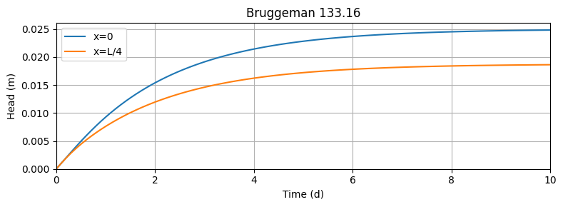
plt.figure(figsize=(8, 3), layout="tight")
plt.plot(t, hx0, label="x=0")
plt.plot(t, hxb2, label="x=L/4")
plt.grid(True)
plt.xlabel("Time (d)")
plt.ylabel("Head (m)")
plt.title("Bruggeman 133.16")
plt.xlim(t[0], t[-1])
plt.ylim(0.0)
plt.legend();
Steady state solution (133.17)#
bruggeman_133_17
\[\begin{split}
\begin{aligned}
\varphi{\left(x,b,k,D,p \right)} &= \frac{p \left(b^{2} - x^{2}\right)}{2 D k} \\
\end{aligned}
\end{split}\]
bruggeman_133_17?
Drainage to canals#
This equation can be used to model drainage to drains and canals.
Results are equal to Krayenhoff van de Leur - Maasland (e.g.: ‘Cultuurtechnisch Vademecum’, 1988, page 523).
mlconf = tft.ModelXsection(naq=1, tmin=1e-3, tmax=1e3)

left = tft.XsectionMaq(
    mlconf,
    -np.inf,
    -b,
    kaq=k,
    z=[0, -D],
    Saq=S,
    topboundary="phreatic",
)
inf = tft.XsectionMaq(
    mlconf,
    -b,
    b,
    kaq=k,
    z=[0, -D],
    Saq=S,
    # c=c,
    topboundary="phreatic",
    tsandN=[(0.0, p)],
)
right = tft.XsectionMaq(
    mlconf,
    b,
    np.inf,
    kaq=k,
    z=[0, -D],
    Saq=S,
    # c=c,
    topboundary="phreatic",
)

d = -1e-3
hls_left = tft.River1D(mlconf, xls=-b + d, tsandh=[(0, 0.0)], layers=[0])
hls_right = tft.River1D(mlconf, xls=b - d, tsandh=[(0, 0.0)], layers=[0])

mlconf.solve()
self.neq  6
solution complete
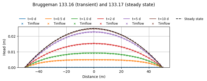
x = linspace(-b, b, 51)
t_steps = [0, 0.5, 1.0, 2, 5, 10]  # time steps in days

fig, ax = plt.subplots(figsize=(8, 3), layout="tight")
for t in t_steps:
    ht = bruggeman_133_16(x, t, b, S, k, D, p)
    (p0,) = ax.plot(x, ht, label=f"t={t} d")
    ax.plot(
        x,
        mlconf.headalongline(x, np.zeros_like(x), t)[0, 0],
        label="Timflow",
        marker="x",
        linestyle="none",
        markersize=4,
        color=p0.get_color(),
    )

h_ss = bruggeman_133_17(x, b, k, D, p)
ax.plot(x, h_ss, label="Steady state", color="k", linestyle="--")

ax.grid(True)
ax.set_xlabel("Distance (m)")
ax.set_ylabel("Head (m)")
ax.set_title("Bruggeman 133.16 (transient) and 133.17 (steady state)", y=1.45)
ax.set_ylim(0.0)
ax.legend(loc=(0, 1), ncol=7, fontsize="small", frameon=False);