128.0x: Tidal fluctuation of open water.#
This notebook shows comparisons of tidal wave propagation in a ‘Timflow’ ModelXsection against known formulas from literature (Bruggeman, 1999: Analytical solutions of geohydrological problems).
Three situations are shown:
Bruggeman 128.01: tidal fluctation of open water, in a confined aquifer with open boundary at x=0
Bruggeman 128.03: tidal fluctation of open water, in a leaky aquifer with open boundary at x=0
Bruggeman 128.04: tidal fluctation of open water, in a leaky aquifer with entry resistance at x=0
import matplotlib.pyplot as plt
import numpy as np
import timflow.transient as tft

from bruggeman.flow1d import bruggeman_128_01, bruggeman_128_03, bruggeman_128_04
View the functions. Since the latter equation is the most generic one (with the others being more specific), we will show that one:
bruggeman_128_04
View the docstring to get a description of the input parameters
help(bruggeman_128_04)
Help on function bruggeman_128_04 in module bruggeman.flow1d:

bruggeman_128_04(x: float | numpy.ndarray[tuple[typing.Any, ...], numpy.dtype[numpy.float64]], t: float | numpy.ndarray[tuple[typing.Any, ...], numpy.dtype[numpy.float64]], h: float, S: float, k: float, D: float, tau: float, c: float, w: float) -> float | numpy.ndarray[tuple[typing.Any, ...], numpy.dtype[numpy.float64]]
    Tidal fluctuation open water, leaky aquifer with entrance resistance (x = 0).

    From Bruggeman 128.04

    Parameters
    ----------
    x : float or ndarray
        Distance from the boundary [m]
    t : float or ndarray
        time [d]
    h : float
        amplitude of tidal fluctuation [m]
    S : float
        storage coefficient [-]
    k : float
        hydraulic conductivity [m/d]
    D : float
        aquifer thickness [m]
    tau : float
        tidal period [d]
    c : float
        leakance [d]
    w : float
        entry resistance at x=0 [d]

    Returns
    -------
    head : float
        head in the aquifer at distance x and time t [m]
Set up the comparison in timflow#
The analytic solution is for a river with varying head that has been varying for ever.
In timflow, head is simulated for several days to get the model to spin-up.
By using a sine function, the head starts at zero (as should be the case in Timflow).
def head_river(h, t, tau, tp=0):
    return h * np.sin(2 * np.pi * (t - tp) / tau)
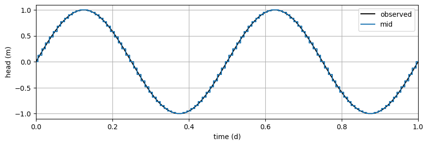
Below the sine (water level on river) is split into steps as shown in the example How to model a fluctuating head boundary from the timflow documentation. We use a small timestep ($\Delta t$)
# Parameters of tidal wave
tau = 0.5  # tidal period, d
h_tidal = 1  # amplitude of tidal fluctuation, m
tmax = 5  # day
delt = 0.01  # day
t = np.arange(0, tmax, delt)
hexact = head_river(h_tidal, t, tau)
hmid = 0.5 * (
    head_river(h_tidal, t - delt / 2, tau) + head_river(h_tidal, t + delt / 2, tau)
)
tmid = np.hstack((0, 0.5 * (t[:-1] + t[1:])))
# plot
plt.figure(figsize=(10, 3))
plt.plot(t, hexact, "k", label="observed")
plt.step(tmid, hmid, where="post", label="mid")
plt.xlim(0, 1)
plt.xlabel("time (d)")
plt.ylabel("head (m)")
plt.legend()
plt.grid()
Bruggeman 128.01 - Confined, no entry resistance#
Create the Timflow model for comparison with Bruggeman 128.01 (confined, no entry resistance).
In this example, we use the 1D inhomogeneities because of the nice plotting. The same result could be reached with a ‘normal’ Timflow model.
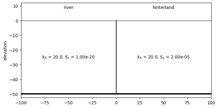
In all the Timflow models, the left-hand inhomogeneity (river) is shown for illustration purposes. That inhomogeneity is only created to satisfy the requirement of ModelXsection to have inhoms for $-\infty<x<\infty$.
The hydraulic boundary river_hls is modeled as a River1D at x=0.
# parameters
k = 20.0  # hydraulic conductivity, m/d
H = 50.0  # thickness of aquifer, m
T = k * H  # transmissivity, m^2/d
S = 0.001  # storage coefficient of aquifer, [-]

Saq = S / H  # specific storage [1/m]
ml = tft.ModelXsection(naq=1, tmin=1e-4, tmax=1e2)

riv = tft.XsectionMaq(
    model=ml,
    x1=-np.inf,
    x2=0,
    kaq=k,
    z=[0, -H],
    Saq=1e-20,
    Sll=1e-20,
    topboundary="confined",
    name="river",
)

land = tft.XsectionMaq(
    model=ml,
    x1=0,
    x2=np.inf,
    kaq=k,
    z=[0, -H],
    Saq=Saq,
    topboundary="confined",
    name="hinterland",
)

# Use a small offset to avoid a singular matrix.
small = 1e-5

river_hls = tft.River1D(
    model=ml, xls=0 - small, tsandh=list(zip(tmid, hmid, strict=True))
)


ml.solve()

ax = riv.plot(params=True, names=True, labels=False)
land.plot(ax=ax, params=True, names=True, labels=False)
river_hls.plot(ax=ax)
ax.set_xlim(-100, 100)
ax.set_ylim(ymax=12);
self.neq  3
solution complete
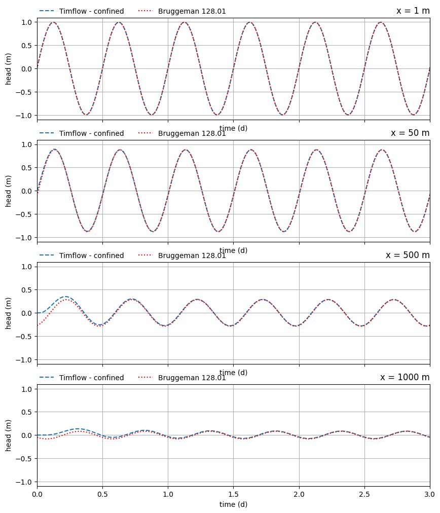
Let’s compare the head at several locations.
As can be seen from the lowest graph $x = 500$, the timflow model needs some spinup time, but after a few days the graphs are similar.
xlocs = [1, 50, 500, 1000]
tp = t

f, axes = plt.subplots(
    len(xlocs), 1, figsize=(10, 3 * len(xlocs)), sharex=True, sharey=True
)

for i in range(len(xlocs)):
    h = ml.head(xlocs[i], 0, tp)
    axes[i].plot(tp, h[0], label="Timflow - confined", linestyle="--")

    h_128_01 = bruggeman_128_01(xlocs[i], tp, h_tidal, S, k, H, tau)
    axes[i].plot(tp, h_128_01, "r", label="Bruggeman 128.01", linestyle=":")

    axes[i].set_title(f"x = {xlocs[i]} m", loc="right")
    axes[i].legend(loc=(0, 1), frameon=False, ncol=2)
    axes[i].grid()
    axes[i].set_xlabel("time (d)")
    axes[i].set_ylabel("head (m)")
    axes[i].set_xlim([0, 3])
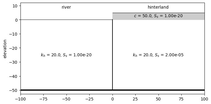
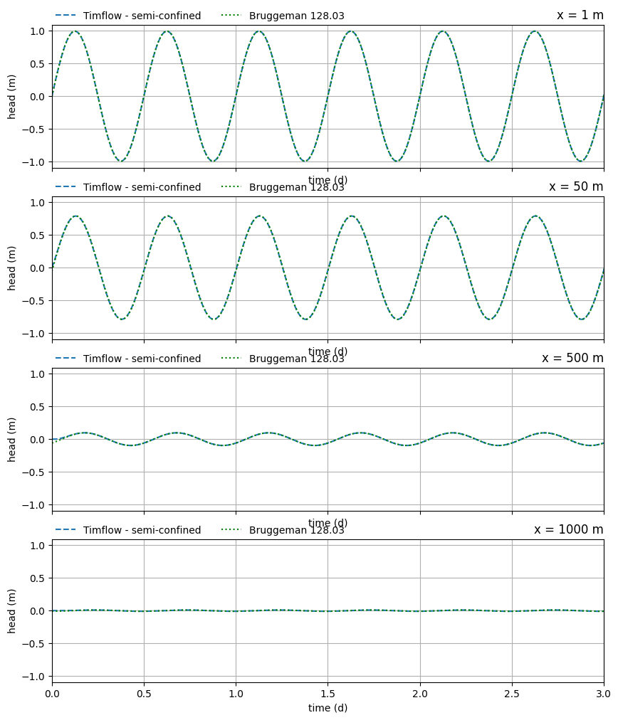
Bruggeman 128.03 Leaky, no entry resistance#
Create a Timflow model for comparison with Bruggeman 128.03 (leaky, no entry resistance).
# Additional parameters for this model:
c = 50  # leakage factor, d

# The model
ml2 = tft.ModelXsection(naq=1, tmin=1e-4, tmax=1e2)

riv2 = tft.XsectionMaq(
    model=ml2,
    x1=-np.inf,
    x2=0,
    kaq=k,
    z=[0, -H],
    Saq=1e-20,
    Sll=1e-20,
    topboundary="confined",
    name="river",
)

land2 = tft.XsectionMaq(
    model=ml2,
    x1=0,
    x2=np.inf,
    kaq=k,
    z=[5, 0, -H],
    c=c,
    Saq=Saq,
    topboundary="semi",
    name="hinterland",
)

# Use a small offset to avoid a singular matrix.
small = 1e-5

river_hls2 = tft.River1D(
    model=ml2, xls=0 - small, tsandh=list(zip(tmid, hmid, strict=True))
)


ml2.solve()

ax = riv2.plot(params=True, names=True, labels=False)
land2.plot(ax=ax, params=True, names=True, labels=False)
river_hls2.plot(ax=ax)
ax.set_xlim(-100, 100)
ax.set_ylim(ymax=12);
self.neq  3
solution complete
Again, compare heads at several locations.
xlocs = [1, 50, 500, 1000]
tp = t

f, axes = plt.subplots(
    len(xlocs), 1, figsize=(10, 3 * len(xlocs)), sharex=True, sharey=True
)

for i in range(len(xlocs)):
    h = ml2.head(xlocs[i], 0, tp)
    axes[i].plot(tp, h[0], label="Timflow - semi-confined", linestyle="--")

    h_128_03 = bruggeman_128_03(xlocs[i], tp, h_tidal, S, k, H, tau, c)
    axes[i].plot(tp, h_128_03, "g", label="Bruggeman 128.03", linestyle=":")

    axes[i].set_title(f"x = {xlocs[i]} m", loc="right")
    axes[i].legend(loc=(0, 1), frameon=False, ncol=2)
    axes[i].grid()
    axes[i].set_xlabel("time (d)")
    axes[i].set_ylabel("head (m)")
    axes[i].set_xlim([0, 3])
Bruggeman 128.04 Leaky, with entry resistance#
Create a Timflow model for comparison with Bruggeman 128.04 (leaky, with entry resistance at x=0).
The entry resistance is added to the River1D river_hls by adding the keyword argument res=w.
# Additional parameters for this model:
w = 20  # entry resistance at x=0, d

# The model
ml3 = tft.ModelXsection(naq=1, tmin=1e-4, tmax=1e2)

riv3 = tft.XsectionMaq(
    model=ml3,
    x1=-np.inf,
    x2=0,
    kaq=k,
    z=[0, -H],
    Saq=1e-20,
    Sll=1e-20,
    topboundary="confined",
    name="river",
)

land3 = tft.XsectionMaq(
    model=ml3,
    x1=0,
    x2=np.inf,
    kaq=k,
    z=[5, 0, -H],
    c=c,
    Saq=Saq,
    topboundary="semi",
    name="hinterland",
)


# Use a small offset to avoid a singular matrix.
small = 1e-5

river_hls3 = tft.River1D(
    model=ml3,
    xls=0 - small,
    tsandh=list(zip(tmid, hmid, strict=True)),
    res=w,
)

ml3.solve()

ax = riv3.plot(params=True, names=True, labels=False)
land3.plot(ax=ax, params=True, names=True, labels=False)
river_hls3.plot(ax=ax)

ax.set_xlim(-100, 100)
ax.set_ylim(ymax=12);
self.neq  3
solution complete
xlocs = [1, 50, 500, 1000]
tp = t

f, axes = plt.subplots(
    len(xlocs), 1, figsize=(10, 3 * len(xlocs)), sharex=True, sharey=True
)

for i in range(len(xlocs)):
    h = ml3.head(xlocs[i], 0, tp)
    axes[i].plot(tp, h[0], label="Timflow - leaky + entry resistance", linestyle="--")
    h_128_04 = bruggeman_128_04(xlocs[i], tp, h_tidal, S, k, H, tau, c, w)
    axes[i].plot(tp, h_128_04, "k", label="Bruggeman 128.04", linestyle=":")
    axes[i].set_title(f"x = {xlocs[i]} m", loc="right")
    axes[i].legend(loc=(0, 1), frameon=False, ncol=2)
    axes[i].grid()
    axes[i].set_xlabel("time (d)")
    axes[i].set_ylabel("head (m)")
    axes[i].set_xlim([0, 3])
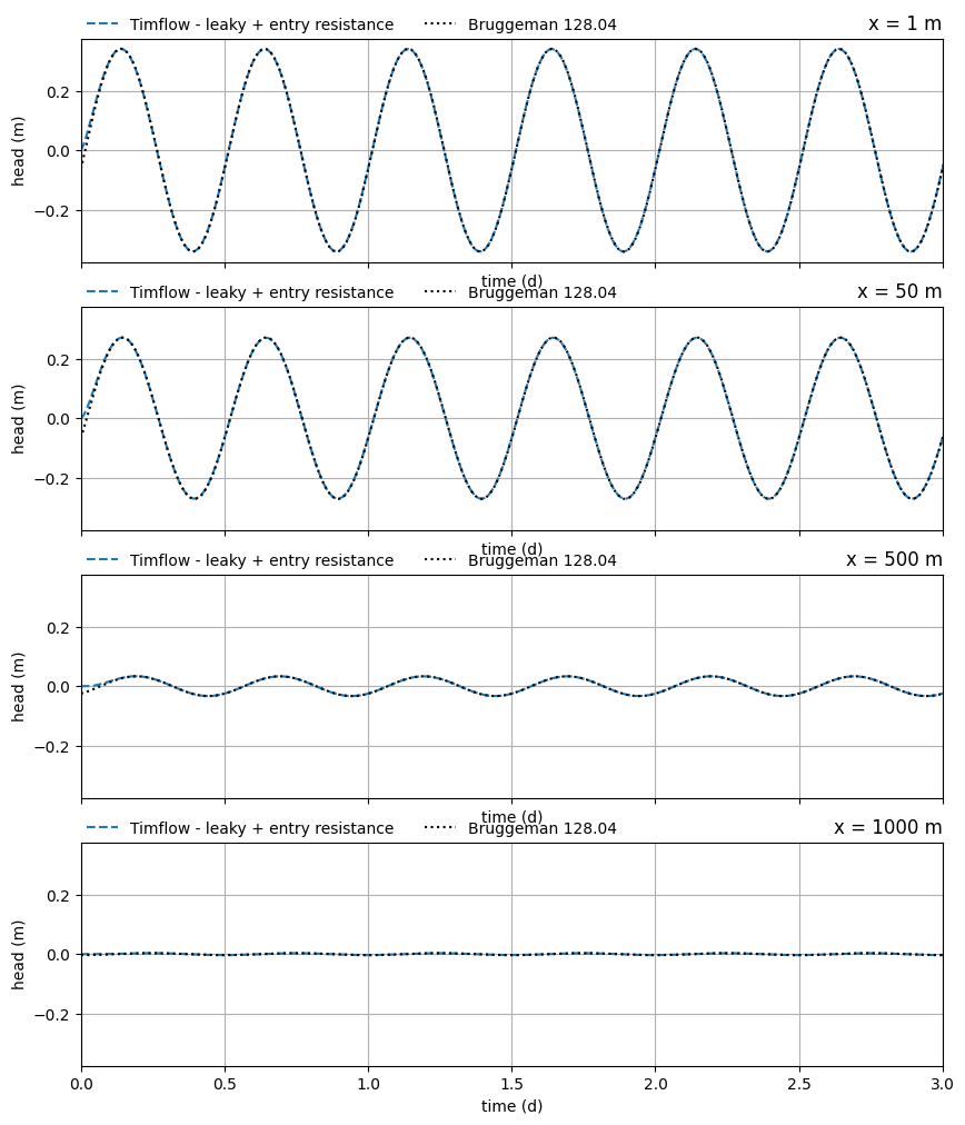
As can be seen, all three cases are replicated accurately after approximately 2 days spinup time.
In the case with entry resistance, the head in the aquifer is already considerably damped compared to the open water fluctuation, even at a small distance (x=1 m).
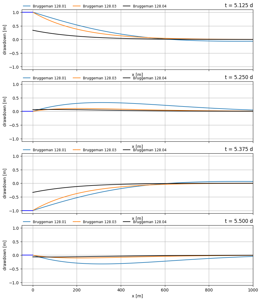
Comparison of the three equations#
Below is a comparison shown between the three equations.
x = np.linspace(0, 1000, 101)
y = np.zeros_like(x)
tg = (10 + np.array([0.25, 0.5, 0.75, 1])) * tau  # time in days

f, axes = plt.subplots(
    len(xlocs), 1, figsize=(10, 3 * len(tg)), sharex=True, sharey=True
)


for i in range(len(tg)):
    h_128_01 = bruggeman_128_01(x, tg[i], h_tidal, S, k, H, tau)
    axes[i].plot(x, h_128_01, label="Bruggeman 128.01", linestyle="-")
    h_128_03 = bruggeman_128_03(x, tg[i], h_tidal, S, k, H, tau, c)
    axes[i].plot(x, h_128_03, label="Bruggeman 128.03", linestyle="-")
    h_128_04 = bruggeman_128_04(x, tg[i], h_tidal, S, k, H, tau, c, w)
    axes[i].plot(x, h_128_04, "k", label="Bruggeman 128.04", linestyle="-")

    h_riv = head_river(h_tidal, tg[i], tau)
    axes[i].plot([-50, 0], [h_riv, h_riv], "b")

    axes[i].legend(loc=(0, 1), frameon=False, ncol=6, fontsize="small")
    axes[i].set_xlabel("x [m]")
    axes[i].set_ylabel("drawdown [m]")
    axes[i].grid()
    axes[i].set_title(f"t = {tg[i]:.3f} d", loc="right")
    # axes[i].set_ylim(0, h_step * 1.2)
    # axes[i].axvline(0, color="grey", linewidth=3)

    axes[i].set_xlim(-50, 1000)