126.33: Steady state after step head change.

import matplotlib.pyplot as plt
import numpy as np
import timflow.transient as tft

from bruggeman.flow1d import bruggeman_126_33

View the function.

bruggeman_126_33

\[\begin{split} \begin{aligned} \lambda &= \sqrt{D c k} \\ \varphi{\left(x,h,k,D,c,w \right)} &= \frac{h \lambda e^{- \frac{x}{\lambda}}}{k w + \lambda} \\ \end{aligned} \end{split}\]

View the docstring to get a description of the input parameters

help(bruggeman_126_33)

Help on function bruggeman_126_33 in module bruggeman.flow1d:

bruggeman_126_33(x: float | numpy.ndarray[tuple[typing.Any, ...], numpy.dtype[numpy.float64]], h: float, k: float, D: float, c: float, w: float) -> float | numpy.ndarray[tuple[typing.Any, ...], numpy.dtype[numpy.float64]]
    Leaky aquifer with entrance resistance. Steady state after head change.

    From Bruggeman 126.33

    Parameters
    ----------
    x : float or ndarray
        Distance from the boundary [m]
    h : float or ndarray
        Rise of the water table [m]
    k : float
        Hydraulic conductivity [m/d]
    D : float
        Aquifer thickness [m]
    c : float
        Leakance [d]
    w : float
        Entry resistance at x=0 [d]

    Returns
    -------
    head : float
        steady state head in the aquifer at distance x [m]

Define some aquifer parameters.

k = 20.0  # hydraulic conductivity, m/d
D = 50.0  # thickness of aquifer, m
T = k * D  # transmissivity, m^2/d
c = 1000  # leakage factor, d
w = 20  # entry resistance at x=0, d
h_step = 1.0  # head at x=0, m
S = 0.001  # storage coefficient of aquifer, [-]

Saq = S / D  # specific storage [1/m]
Sll = 0.001  # specific storage of leaky layer, [-]

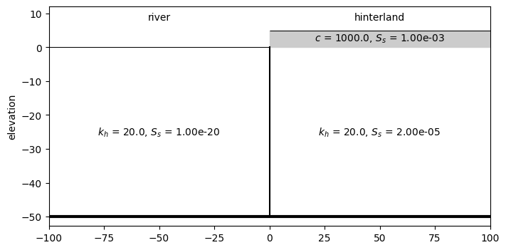
Set up a timflow model.

The ModelXsection to be able to plot the sections, but the same result could be reached with the ‘normal’ ModelMaq model.

# The model
ml = tft.ModelXsection(naq=1, tmin=1e-4, tmax=1e3)

riv = tft.XsectionMaq(
    model=ml,
    x1=-np.inf,
    x2=0,
    kaq=k,
    z=[0, -D],
    Saq=1e-20,
    Sll=1e-20,
    topboundary="confined",
    name="river",
)

land = tft.XsectionMaq(
    model=ml,
    x1=0,
    x2=np.inf,
    kaq=k,
    z=[5, 0, -D],
    c=c,
    Saq=Saq,
    Sll=Sll,
    topboundary="semi",
    name="hinterland",
)

# Use a small offset to avoid a singular matrix.
small = 1e-5

river_hls = tft.River1D(
    model=ml,
    xls=0 - small,
    tsandh=[0, h_step],
    res=w,
)

ml.solve()

ax = riv.plot(params=True, names=True, labels=False)
land.plot(ax=ax, params=True, names=True, labels=False)
river_hls.plot(ax=ax)

ax.set_xlim(-100, 100)
ax.set_ylim(ymax=12)

self.neq  3
solution complete

(-52.75, 12.0)

Compare timflow implementation to the analytical solution from Bruggeman.

x = np.linspace(0, 1000, 101)
y = np.zeros_like(x)
t = np.logspace(-1, 1, 3)

plt.figure(figsize=(10, 3))
for i in range(len(t)):
    h = ml.headalongline(x, y, t[i])
    plt.plot(x, h.squeeze(), label=f"t={t[i]:.2f} d")
    ha = bruggeman_126_33(x, h_step, k, D, c, w)
    plt.plot(x, ha, "k:")
plt.plot([], [], "k:", label="Bruggeman 126.33")
plt.legend(loc=(0, 1), frameon=False, ncol=6, fontsize="small")
plt.xlabel("x [m]")
plt.ylabel("drawdown [m]")
plt.grid()
plt.ylim(0, h_step * 1.2)
plt.axvline(0, color="grey", linewidth=3)
plt.plot([-50, 0], [h_step, h_step], "b")
plt.xlim(-50, 1000)

(-50.0, 1000.0)

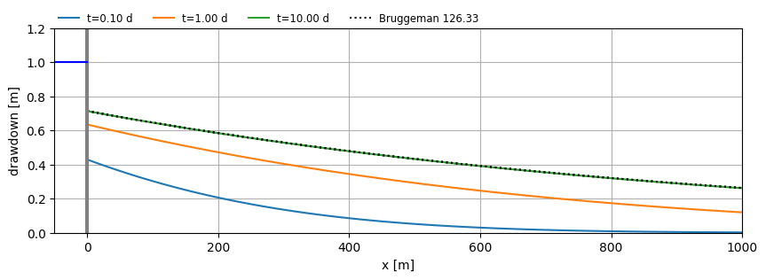
As can be seen from the graph, the storativity causes a delay in reaching the steady-state value. When the storativity approaches zero, the steady-state is immediately reached.

Furthermore, the head in the aquifer never reaches the head in the river, because of the entry resistance.